Surface Triangulations and Quivers

Last time I discussed the ADE classification of finite type quivers. I ended that post with a remark that for quivers with relations, there is no classification that is nearly as nice as the ADE classification, in general we work on a case by case basis.  The particular case I am interested is a class of algebras called 2-Calabi-Yau tilted.  These algebras come up in the study of another class of algebras called cluster algebras, we are not going to focus on that connection here instead I want to focus on an alternative construction that uses Riemann surfaces.

By triangulation I mean a diagram like below

Figure 1 : a triangulation of the disc. 

Concretely, a (non-punctured) triangulated surface is a triple $(S,M,T)$ with $S$ is a oriented Riemann surface with boundary, $M\subset \partial S$ a finite set of points in the boundary, and $T$ a maximal collection of non-crossing curves in $S$ with endpoints in $M$.  We will consider the curves in $T$ up to homotopy and we do not make any restrictions on the number of boundary components.

Figure 2 : a triangulation of the annulus.

Clearly, we are not dividing the surface into exact triangles, hence, these are also referred to as ideal triangulations.

From such a triangulation we can construct a quiver with relations. We denote this quiver $(Q_T, I_T)$, we take the surface as being understood.  Let the set of vertices be indexed by the arcs in $T$.  There is an arrow $i\to j$ in $Q_T$ if the curves $\gamma_i, \gamma_j\in T$ are incident to each other and form part of the boundary of a triangle $\triangle$ such that $\gamma_j$ follows $\gamma_i$ as you walk around the boundary of $\triangle$ in the counter-clockwise direction (recall that the surfaces are oriented). That definition may seem like a word jumble, so consider the following picture

$\gamma_i$ and $\gamma_j$ are point of the boundary of a triangle and $\gamma_i$ precedes $\gamma_j$, so we get an arrow $i\to j$.

At this point we have only constructed $Q_T$.  The ideal $I_T$ is defined to be the composition of any two arrows that are defined by the same triangle.   It is not obvious from this definition, but there are only three types of triangles in a triangulation

• those with only one edge from $T$, which defines no arrows;
• those with two edges from $T$, which defines exactly one arrow;
• and those with three edges from $T$, which defines three arrows.

Only the last contributes to $I_T$.   The algebra associated to $(Q_T, I_T)$ belongs to a class of algebras called 2-Calabi-Yau tilted. The name comes from the fact that these algebras are associated to certain tilting objects in certain 2-Calabi-Yau categories.  I. Reiten gives a good introduction to the details of which objects and which categories here.

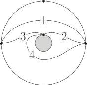
At this point we are ready for examples.  First going back to Figure 1

we get the following quiver

with $I_T = \langle ab, bc, ca\rangle$.  In Figure 2, we hade

which defines the quiver

with $I_T = \langle ab, bc, ca\rangle$.

To clean up the statement of the next theorem, let me introduce one more piece of notation.  Let $\mathcal C$ be the set of all homotopy classes of curves in the interior of $S$ with endpoints in $M$.  The reason for doing this is that the following

Theorem.(BZ) Let $(S,M,T)$ be a triangulation of a surface as given above.  The representations of $(Q_T,I_T)$ are in bijection with $\mathcal C\setminus T$.

The theorem is in fact stronger.  We can define a category with $\mathcal C$ being the objects and morphisms being elementary pivots. Then we actually get an equivalence of categories with the representations of $(Q_T,I_T)$.  I discuss this in detail with additional references here.  The punchline is this, instead of studying the quiver and its corresponding algebra directly, we should be able focus our study on the surface.  For quivers of Dynkin type $A$, which arise as certain triangulations of the disc, this is overkill; but, for other quivers this gives us a new angle to attack their representation theory.  In approximately 2 posts I will give a particular example where the surface presentation is especially useful.

At this point I should mention at least one caveat and 2 possible generalizations of this constructions.  First the caveat.  When defining the arrows, I choose to orient the arrows by traveling the boundary of a triangle in the counter-clockwise direction.  There is no good reason to prefer this direction over clockwise, in fact, many people do use the clockwise direction. Hence, when reading related work using surface triangulations, it is important to look for which convention a person is using.

Now the generalizations.  The simplest generalization is to consider other possible subdivisions of the surface.  Here we required the subdivision to to have 3 boundary segments (at least one from $T$). We can just as easily define $m$-angulations in which the subdivisions have $m$ boundary segments (at least on from $T$).  When the surface is a disc, the resulting algebras are $m$-cluster tilted.

The other possible generalization is to allow the points of $M$ to also belong to the interior of $S$. These surfaces are considered punctured.  The notion of a triangulation must be suitably modified, the details were fully worked out by D. Labardini-Fragoso.  The benefit of the punctured surfaces, beyond having more generality, is that certain triangulations of the punctured disc gives rise to type $D$ quivers. The exceptional Dynkin types $E_6$, $E_7$, and $E_8$ do not occur as triangulations of surfaces.

In the next post I will give an example where the surface realization is used to simplify a calculation.

ADE classification

Last time I introduced the idea of quiver representations, basically, collections of vector spaces and linear maps that are compatible with a given quiver with relations $(Q, I)$.  It turns out that the collection of representations for a fixed quiver  is a Krull-Schmidt category.  This means that we have a notion of direct sums of quiver representations.  It is constructed in the most obvious way, by taking direct sums at each vertex and along the arrows.  For example, it we consider the simple quiver $1 \longrightarrow 2$, then we have the following direct sum of representations

Here I have taken the direct sum at each vertex, producing $\mathbb C^3$, and then identified the last basis element with the the representation $\mathbb C \xrightarrow{1}\mathbb C$.

In practical terms the Krull-Schmidt property means that we can restrict our focus to only the indecomposable representations of $(Q,I)$, those representations that can not be broken into a non-trivial direct sum.   The obvious question is how do I distinguish which representations are indecomposable? In the example given above only the representation $\mathbb C\xrightarrow{1}\mathbb C$.   The larger representation can be broken up into the following direct sum

Where the isomorphism is realized by the pair of matrices $\left(\begin{smallmatrix} 1& i\\0&1\end{smallmatrix}\right)$ and $\left(\begin{smallmatrix} 1& 0\\0&1\end{smallmatrix}\right)$.
(Here I am starting with the original representation and mapping it to the representation with the identity matrix along the arrow.)

The follow up question might be, how many indecomposable representations are there? This question of course requires the question : are there only finitely many indecomposable representations?   Especially as computers get more powerful, the knowledge that there are only finitely many representations would be nice, to identify the indecomposables we would simply need to (get a computer) to enumerate them.   Those algebras that have only finitely many indecomposables are said to be of finite type.

To simplify things I will only consider quivers without relations, that is $I=0$.  With this restriction we get a satisfying though short answer the number questions thanks to P. Gabriel:

Theorem. The path algebra of a quiver has only finitely many indecomposable representations if and only if the underlying graph is a Dynkin diagram of type $A$, $D$, or $E$. 

You may have heard of the Dynkin diagrams before; as the this discussion on MathOverflow shows, they show up in many places across mathematics. The unfortunate result of this theorem is that most quivers will have infinitely many indecomposables.  Of course, the not so unfortunate part is that there is plenty of more mathematics to be done.

So for this restricted case of finite type quivers without relations, how many indecomposables are there?  For type $A_n$ where $n$ is the number of vertices, the indecomposable representations are counted by the $\frac12 n(n+1)$.  For type $D_n$, the number of indecomposables is $n(n-1)$. For types $E_6$, $E_7$, and $E_8$m, the number of indecomposables is 36, 69, and 120 respectively.   In the previous example, that is, $Q$ being $1\longrightarrow2$, there are exactly 3 indecomposables which we can list as
\[\mathbb C\longrightarrow 0,\qquad  \mathbb C\xrightarrow{\ 1\ } \mathbb C,\quad \text{ and } 0 \longrightarrow \mathbb C.\]
I have not said anything about how I generated this  list, that will be a post for a future date.

For quivers with relations the story is much more complicated.  In fact, I don't believe that there is any concise method for determining if an arbitrary quiver with relations is finite representation type. Most work seems to be done in special cases or classes of quivers. Next time I will introduce a class of quivers that are constructed from surface triangulations.  These quivers will not always be finite type, but as a whole have an elegant theory for describing their representations.

Quiver representations

Last time  I introduced the idea of quivers. Basically the idea is that if you want to study algebras and their modules, then picking a nice presentation of those algebras may be useful.  Of course, when stated like this, this is obvious.  No one wants difficult presentations of their abstract objects, but at this point it remains to be seen if quivers actually are nice presentations.

Last time I left out one detail that I should include here so that the following statements are actually true.  I said that we can find a quiver presentation for all* algebras.  Well it turns out that there is some important fine print here.  Primarily, if your algebras is basic and connected; then, there is a unique quiver with relations that we can associate to it, I will come back to this business about relations in a moment.  Why do we want these conditions on the algebra?  I will work backwards.  If your algebra is not connected, then the quiver you would build will not be connected.  This doesn't seem like a big deal, but most of the time we like to work with connected quivers and generalize from there.  The connected condition is mostly a technical condition, at least so far. The basic condition is more important but there is a convenient work around: given an algebra $A$, there is a basic algebra $A^b$ such that the category of $A$ modules and equivalent to the category of $A^b$ modules. This is the concept of Morita equivalence.  I really only want to study modules, so as far as considering all the possible module categories is concerned, quivers will produce everything that I want to consider.

What are these relations on the quiver?  Basically, this is how we introduce additional zero-divisors.  I call the pair $(Q,I)$ a bound quiver where $I$ is some ideal in $\mathbb CQ$ such that $I$ does not contain any arrows (or sums of arrows).  For instance, what if we wanted to only consider the algebra generated by the polynomials with degree 1?  We would consider $\mathbb C[X]/(X^2)$.  In terms of quivers this is $\mathbb CQ/(a^2)$ where we use the identification of $\mathbb C[X]$ with

Figure 1

In this example $a^2 = 0$.  Similarly, we can consider the quiver

Figure 2

and the ideal $I = \langle a_2a_3\rangle$.  In this case, we would consider any paths that contain $a_2a_3$ to be zero, so $a_1a_2a_3 = 0$ in $\mathbb CQ/I$.

The short story of why quivers are a good way to present your algebras is that it immediately gives us a way to present the corresponding modules as quiver representations.  Given a quiver $Q$, a quiver representation is a collection $M$ of vector spaces and linear maps $\{ V_i, \phi_a\}$ where $i\in Q_0$ is a vertex and $a\in Q_1$ is an arrow such that $\phi_a \colon V_{s(a)} \to V_{t(a)}$, that is the linear map associated to $a$ makes sense with the vector spaces at the source and target of the arrow.

If $(Q,I)$ is the bound quiver associated to an algebra, then we require the that the maps associated to paths in $I$ should compose to zero.  Going back to Figure 2 and $I = \langle a_2a_3\rangle$, a quiver representation would be $V_i = \mathbb C$ for $i\in Q_0$ and $\phi_1 = \phi_2 = 1$ and $\phi_3 = 0$. We do not have much choice in which linear maps we can pick for the arrows.  Since each vector space in this representation is one-dimensional, each of the linear maps is multiplication by a constant from $\mathbb C$. We need $\phi_3 \circ \phi_2 = 0$, so either $\phi_3 = 0$ or $\phi_2 = 0$.  So, for instance, $V_i = \mathbb C$ for $i\in Q_0$ and $\phi_a = 1$ for $a\in Q_1$ is not a representation of $(Q,I)$, but, it would be a representation of $Q$ (here we can think of setting $I=0$).

We can of course present quiver representations as diagrams. For instance here two representation of $(Q,I)$ as given above:

Figure 3

In the same way maps between representations are easy to describe as well:

Figure 4

Morphisms of quiver representations $M = \{ V_i, \phi_a\}$ and $N= \{ W_i, \xi_a\}$ are collections of linear maps $\psi_i$ for $i\in Q_0$ such that $\psi_i \colon V_i \to W_i$ and so that all of the obvious squares commute, that is $\psi_i\xi_a = \phi_a\psi_{t(a)}$.

Throughout the rest of these posts, I will always assume that my algebra is finite-dimensional and that the vector spaces in a quiver representation are also finite-dimensional.  The benefit of doing this is that when it gets down to the gritty details of proving stuff or working with concrete representations  everything is vector spaces and matricies.

What we have done is generalize the example of $\mathbb C[X]$ in which all of its modules can be described by a vector space and a particular matrix.  Next time we will talk about some special quivers that deserve a distinguished place in this theory.

Sound problems

Yesterday I finally decided to fix a problem  with my laptop that I had been ignoring for at least a year. Essentially, when I used the volume buttons on my keyboard the volume would change by approximately 25% of its max loudness, so it got loud or quiet very fast.  I could change the volume in smaller increments using the volume slider but I like using the keyboard buttons, so my laptop had essentially 3 volume levels: loud, audible, and mute.  The source of the problem seems to be this bug  and unfortunately upstream (Gnome I think) did not want to spend much, or any, time on fixing this.

Fortunately, after much sleuthing, I found this post on ask Ubuntu, which in turn uses information found on Ubuntu's wiki which unfortunately has removed that page.    The fix boils down to adjusting two lines in a config file:

Fix / Workaround

There are a few variables which control how PulseAudio controls the volume. You can either edit /etc/pulse/default.pa (you'll have to be root to do that) to change the behavior for all users, or copy that file to ~/.pulse/default.pa and then edit that file, to change behavior for the current user only.

Open the file mentioned above. Find the row saying "load-module module-udev-detect" and change it to:

load-module module-udev-detect ignore_dB=1

and I also needed

Find the row saying "#load-module module-alsa-sink" and change it to:

load-module module-alsa-sink control=PCM

Of course you may be wondering why I am blogging about something like this.  Well, simply put this is mostly intended to be a personal trail of breadcrumbs.  More math will be coming later this afternoon.

Quivers

The next couple of weeks will be an experiment to help get me blogging.  This coming Friday I am giving a talk on "Representation theory via surfaces"

We will discuss the representation theory of finite dimensional algebras by using quiver theory and surface triangulations.  These methods allow us to give concrete descriptions of modules over finite dimensional algebras and open the theory to rich combinatorial methods.  We will focus on the algebras of finite representation type and the related tilted algebras of global dimension two.   

Today I want to start with some background and my perspective on what representation theory is and why you might want to use quivers to study it.

Of course deciding where to start is always troublesome.  We will start with Jordan normal form.  If you have done any linear algebra past a basic first semester course, you will have run into Jordan normal form. What you may not have run into is the fact this completely describes the representation theory of the polynomial ring $\mathbb C[X]$, that is using Jordan normal form we can describe all of the modules over $\mathbb C[X]$.  You can actually find the "proof" of this in Dummit and Foote so it is likely that you have seen this but didn't realize it. Basically the idea goes like this, given an $n$-dimensional  ($\mathbb C$) vector space $V$ and an $n\times n$ matrix $A$, we can have a polynomial
    $$p(x) = a_0 + a_1x + \cdots a_m x^m$$
act on $V$ by defining $$p(x) \cdot v = a_0 v + a_1 A\cdot v + \cdots a_m A^m \cdot v.$$   The standard exercise is to show that this is in-fact the only way for $\mathbb C[X]$ to act on a vector space.   Putting this together with Jordan normal form means that we have a complete description of how $\mathbb C[X]$ acts on vectors spaces and further we have a method to determine when two seemingly different actions are the same: the actions are distinct (up to an isomorphism) if and only if Jordan normal form of the corresponding matricies are the same.

The lesson to take from the Jordan normal form business is that by picking an appropriate basis  on $V$ we can read important information about the action of $\mathbb C[X]$.   Quivers are a method for choosing a special presentation of the algebra we want to study and in turn (as we will see later) this will dictate a special presentation for the corresponding module we want to study. For $\mathbb C[X]$ we have the following presentation

Figure 1

We need some terminology and notation before we can formalize the connection between the above picture and $\mathbb C[X]$.  A quiver $Q$ is simply a directed graph, so $Q = (Q_0,Q_1)$ where $Q_0$ is a set of vertices (my quivers are always finite, so I will generally use natural numbers) and $Q_1$ is the collection of arrows.   When needed we also have the maps $s, t\colon Q_1 \to Q_0$ that read off the source and target of an arrow. A path in a quiver is simply a sequence of arrows $a_1a_2\cdots a_t$ in $Q$ such that $t(a_i) = s(a_{i+1})$.  For example consider

Figure 2

Then $a_1a_2$ is a path in $Q$, so is $a_1a_3^5a_2$, where $a_3^5$ simply means to repeat $a_3$ five times.   We also define "stationary paths" at each vertex in $Q$, denoted $e_i$. These are paths with $s(e_i) = t(e_i) = i$ and containing no arrows.  With this notation, we can define the path algebra $\mathbb CQ$ of a quiver to be the

1. the $\mathbb C$ vector space spanned by the paths in $Q$ (really any field can be used, but we might as well use a nice field),
2. with multiplication given by concatenation of paths when it makes sense or zero otherwise,
3. the identity $1$ is given by the sum of the stationary paths,  $e_1+\cdots + e_n$.

 This is of course a good time for an example.

Figure 3

 Let $Q$ be the quiver in Figure 3, then some elements in $\mathbb CQ$ would be 

\[\begin{aligned}
a_1,&\\
2a_2,&\\
i a_1 + a_1a_2,&
\end{aligned}\]

and we could consider the multiplication by $a_1$ on each of these elements
\[\begin{aligned}
a_1 \cdot a_1 &= 0\\
a_1 \cdot 2a_2 &= 2a_1a_2\\
a_1 \cdot (i a_1 + a_1a_2) &= 0
\end{aligned}\]
With this machinery now built we can be explicit about how  $\mathbb C[X]$  is isomorphic to path algebra $\mathbb CQ$ of

.

Let $p(X) = c_0 + c_1 X + \cdots c_m X^m\in \mathbb C[X]$, then isomoprhism $\mathbb C[X] \cong \mathbb CQ$ is given by
\[p(x) \mapsto c_0 1+ c_1 a + \cdots c_m a^m.\]

In general, we can do this for all* algebras.  A proof of this claim can be found at the end of chapter 2 in Elements of the Representation Theory of Associative Algebras I by Assem, Simson, and Skowronski.  Next time I will talk about how to present modules in terms of quivers. 

NYT says drop out

Let met start by saying that I agree that there are situations in which a person need not go to college but articles like this from the New York Times are dangerous.  The author, Alex Williams, repeatedly cites the examples of people like Steve Jobs or Mark Zuckerberg but fails to note that these people did not single handedly build their multi-million dollar businesses. Facebook, for example, was co-founded with Eduardo Saverin and Chris Hughes who  did actually finish their degrees at Harvard.  Andrew McCollum, another founder of Facebook, did dropout for a little more than a year but quickly went back and finished a degree in computer science.  Further, I suspect that a college drop out might have difficulty getting a job at Apple or Facebook today.

What about the other people that Alex mentions?  The article starts off talking about Benjamin Goering who dropped out of college and is now working at LiveFyre.  Several of the leadership positions are filled with college graduates.

Most if not all of the people mentioned got into college and then dropped out.  Beyond that, the  big familiar names like Steve Jobs, Bill Gates,  and Mark Zuckerberg were at elite schools.  As far as we know these people did not flunk out, they are drop out because they are not engaged/challenged in the classroom.  These are people that can very easily return to college if they want to.  The un-college perspective is coming from a very privileged perspective of people that have at worst postponed college and seems to be coming almost entirely from people in technology, specifically programming and social applications.  Show me the (young) engineer that is making six figures. Or any other technical field for that matter. The un-college movement would be more convincing if it had a more diverse set of role-models.  It is one thing for Mr. Ellsberg to say “I know people with dog-walking businesses who make six figures” and another to actually name and celebrate this person.

Finally, are we really going to argue about the value of a liberal arts education.

Last year, an anonymous academic who called himself Professor X, published “In the Basement of the Ivory Tower,” which argued that future police officers and nurses need not be force-fed Shakespeare.

This is short-sighted and obnoxious.  Art, literature, math, and science help the the aforementioned police officers and nurses understand and empathize with the people they are helping.  The liberal arts expose us to ethics and provide the means to rigorously analyze our own beliefs and understand why the world is the way it is today.

Not every person needs or should go to college.  It seems that the bulk of the argument the un-college movement is based on the debt that many students take on in order to go to school.  Perhaps the biggest issue is the number of students that take on this debt but never finish a degree or take 6 or more years to complete the degree.  This is largely a failure of the school system prior to getting to college, students enter woefully unprepared and with poor guidance as to what they are doing there.    We should not tell students that it is sufficient to just go to school, which I fear many high school teachers and guidance councilors are saying.  College does not equal a job. College is simply a means to an education.  If you have a job in mind that requires a particular education/skill set, then by all means go to college. Of course there may be other ways to get that skill set.  If you simply like learning stuff, then go to college. This is what we should be telling people.  We should not be sending people to college with the goal to "figure it out," there are cheaper ways to do that, or at least there should be a cheaper way, perhaps the next college dropout can find that for us.